2026-10-19 CVXOPT Scribe
Recap: Approximation and Fitting
Last class we saw that approximation/fitting/estimation all look like a norm minimization problem.
We saw two equivalent notations - statistical and book.
$$ \text{minimize}_{\beta} \|XB- y\| $$This is the standard notation used in statistics and machine learning. Our data is $(x, y)$ pairs that we stack and represent as $X, y$. $\beta$-s are the model parameter that we are trying to find.
$$ \text{minimize}_{x} \|Ax - b\| $$This is the obscure notation used by the book where the data is represented using $A$ and $x$ is the variable that we are trying to optimize.
We also say that it is customary to denote this using residuals and our problem becomes residual minimization.
$$ \|X\beta - y\| = \|r\| $$Our modeling of the data is additive. The statistical interpretation of regression is that
$$ Y = f(X, \beta) + \varepsilon $$Where $\varepsilon \sim F$ is some additive error term. Each of these $\varepsilon$ are i.i.d.
Types of norms
Then we discussed the different types of norms.
- $\|\cdot\|_2$ is the standard euclidean norm. We usually square it to make our lives easier when differentiating
- $\|\|_1$ the 1-norm is robust to outliers
- $\|\|_\infty$ Chebyshev norm is the maximum error of one of the coordinates
More generally we say that we can replace the norm with a penalty function $\phi$ and write our problem as $\sum_i^n \phi(x_i^T \beta - y_i)$
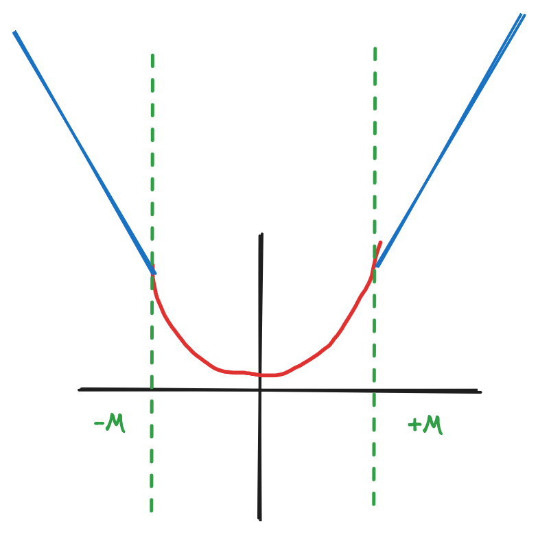
An example of a nice loss function is Huber loss which is $\ell^2$ close to 0 and $\ell^1$ outside outside.
Regularization
So far, we’ve only had a single objective i.e $\|Ax-b\|$ but what if in addition to this we also want $\|x\|$ to be small as well?
This is a bi-criterion problem. How do we solve this? You can even have the norms to be different. They most probably are in terms of dimension anyways.
You can independently plot the two curves and try to find an intersection. $\|x\|$ is not very interesting as the minimizer is 0. We are interested in the other case where out of all the smallish minimizer of $\|Ax-b\|$ which has the smallest norm?
We formulate this using Regularization.
We form a new problem
$$ \text{minimize} \|Ax-b\| + \gamma \mathcal{R}(x) $$Where $\mathcal{R}$ is the minimizer that we’re gonna use.
More generally we can think of the minimizer as a secondary goal that that we want to achieve that may possibly conflict with the primary one. This creates a trade-off that we have to make.
Examples of regularizers
$\ell^2$ regularizer or Tychonov regularizer
Our new objective function is
$$ \text{minimize}_x \|Ax - b\| + \|x\|_2 $$What does this actually do? We know that all norms try to suck $x$ towards 0. But $\ell^2$ have heavy penalties on large values of $x$. So it is pretty much impossible to have that as the optimal point.
We’re essentially asking the minimizer to be very close to 0 if possible.
$\ell^1$ regularizer or sparsity regularizer
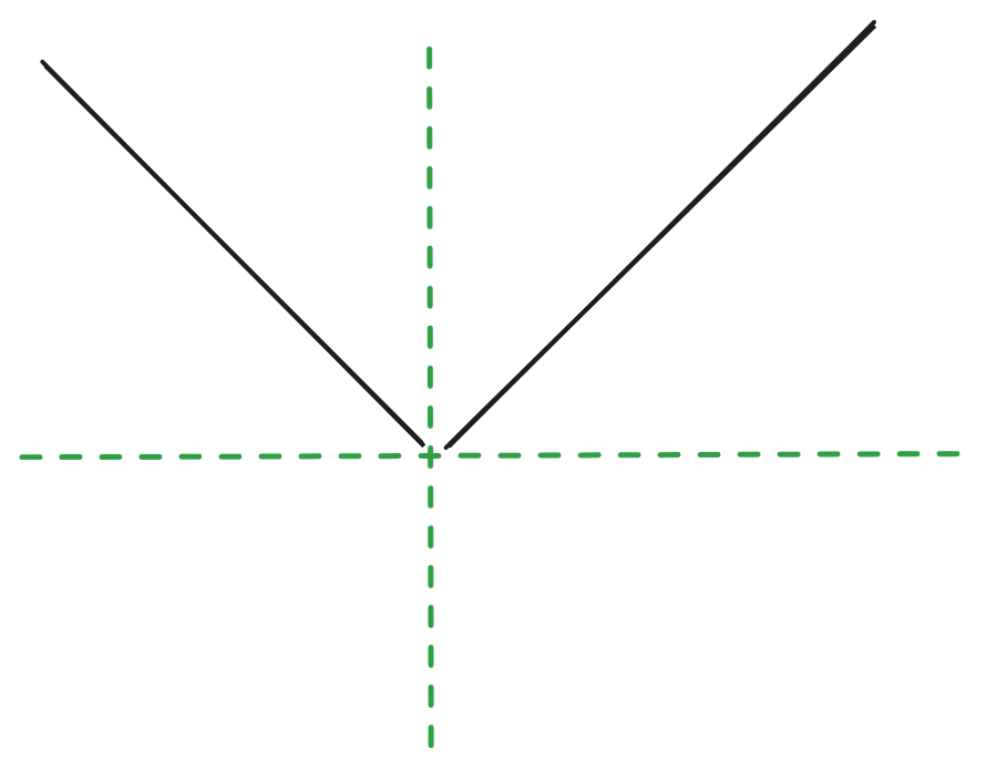
$\ell^1$ equally weights all the values. The gradient is the same regardless of how big $x$ gets. So larger values are not essentially penalized but it is only 0 when $x$ is 0. Hence values close to $0$ are equally unhappy as values that are very far away. This causes the to be very aggressively moved towards 0. This is why it is called sparsity regularizer as you get $x$-s that have exactly 0s in many of their dimensions.
This different from $\|X\beta - y\|_1$ here the entire residual is sparse not $\beta$.
$\|Ax - b\| + \gamma \mathcal{R}(x)$ makes the $x$-s sparse.
Polynomial Regression
Why only use first order terms of the data? Why not more? What if you think the higher order terms are better predictors that the first order one? This is polynomial regression.
This is still linear in the parameters. We are only using higher order terms of the data. You can just think of these higher order terms as just extra dimensions.
We create the following matrix
$$ X = \begin{bmatrix} x_1 & x_1^2 & x_1^3 & \ldots & x_1^k \\ \ldots & \ldots & \ldots & \ldots & \ldots \\ x_n & x_n^2 & x_n^3 & \ldots & x_n^k \\ \end{bmatrix} $$But how do we determine $k$? Too small of a $k$ leads to underfitting and too large of a $k$ leads to overfitting.
To solve this we use regularization
$$ \text{minimize}_\beta \| y - X\beta \|_2^2 + \gamma \|\beta\|_2^2 $$The euclidean norm is a smoother. It indiscriminately disincentivizes larger $\beta$s. So the effect of all the dimensions are dampened.
If we had used $\ell^1$, which we have already seen to be very aggressive, pushes a lot of $\beta$s to be 0.