2026-10-18

2026/09/17 CVXOPT Scribe

$\newcommand{\R}{\mathbb{R}}$ $\newcommand{\E}{\mathbb{E}}$ $\newcommand{\qq}{\quad\quad}$

Operations that preserve Convexity of a function

Non negative weighted sums

Suppose some convex functions $f_i: C_i \subseteq \R^n \rightarrow \R,\qq i=1,\ldots,m$.

Then,

is guaranteed to be convex

Proof Sketch

You can easily prove this by the $\theta, 1-\theta$ definition of convex functions.

$\theta, 1-\theta$ definition may be hard to work with when dealing with complex functions, but in case of composing smaller functions it makes the proof quite easy.

Composition with an affine mapping

If $f: C \subseteq \R^n \rightarrow \R$ is convex then $\tilde{f} = f(Ax-b),\qq A\in\R^{n\times m}, b\in\R^n, x\in\R^m$ is also convex.

Pointwise maximum

Suppose you have two convex functions $f_1, f_2 : C\subseteq \R^n \rightarrow \R$ then

is also convex

Proof Sketch

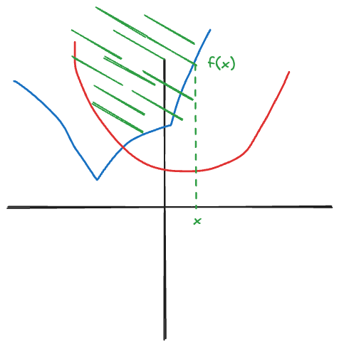
Think about the epigraph of the new function. You’ll see that the convex property is satisfied everywhere.

We can extend this to arbitrary intersection of convex functions

Examples

• Point-wise maximum of Affine functions or a Piecewise-linear function is a convex function
  • $\max\{a_1^T x + b_1, \ldots, a_n^T x + b_n\}$
• Maximum eigenvalue of a symmetric matrix
  • $f(X) = \lambda_{\max}(X) = \sup\{y^TXy:\|y\|_2 = 1\},\qq X\in S^n$
  • This kinda looks like the operator norm of $X$

Composition

Suppose you have two convex functions $h: D \subseteq \R^k \rightarrow \R^n$ and $g: C \subseteq \R^n \rightarrow \R$. Let $D, C, \R^n$ be all convex sets.

Then we define a new function $f = g \circ h (x) = g(h(x))$.

The convexity of $f$ is not so simple to determine as the above cases.

For simplicity assume that $h, g$ are differentiable. Then we can twice-differentiate $f$ to get

As $g, h$ are convex functions we know that,

• $g'' \ge 0$
• $h'' \ge 0$

As $h'(x)^2 \ge 0$, the first term is positive. So for $f'' \ge 0$, we need $g'(h(x)) \ge 0$.

This would require $g$ to be monotonically increasing.

We could also have $g$ be monotonically decreasing and $h$ be concave to have $f$ be convex.

Notice that though we assumed differentiability, the final rules don’t involve any derivatives. Hence, we can consider these to be true for even non-differentiable $g, h$.

Monotonicity of multivariate functions

To determine if a function is increasing/decreasing in $\R^n$, we fix all other coordinates to be constant and just move along one. We do this for all coordinates and notice if the function increases/decreases. If it increases/decreases on all cases we call it monotonically increasing/decreasing.

Vector case

If the inside function is a vector-valued function, then

The same rules apply recursively for each argument of $h$

Proof

As $g$ is convex we have $\mathbf{H}_g \succeq 0$ as $g$ is convex. Then we have $h^T \mathbf{H}_g h \ge 0$.

Jensen’s Inequality

The convex condition

is called Jensen’s inequality.

If $f$ is a convex function, then

$f(\E[x]) \le \E(f(x))$

This very useful machine learning.

If we have $f(x) = -\ln(x)$ then $\E[-\ln(x)]$ gives a global under-estimator of $-\ln(\E(x))$ which might be hard.

If we think of the $\theta$ in $-\ln[(1-\theta)x + \theta y]$ as a probability, then this is a Bernoulli distribution. Our convex function becomes a probability distribution.

Ch. 4 Convex Optimization Problems

The general form of an optimization problem is

Let the feasible set be called $\mathscr{F} = \{x : g_i(x) \le 0, h_j(x) = 0, i\in[m], j\in[p]\}$

Then the optimal point $p^* = \inf_{x\in \mathscr{F}}\{f(x)\}$ and the optimal point $x^* = \arg\inf_{x\in \mathscr{F}}\{f(x)\}$.

Notice that when $p^* = \infty$ we don’t have any feasible points. When it is $-\infty$ the objective function is unbounded below.

Local Optimum

We call $x$ the local optimum if

Convex optimization Problem

such that $f$ is convex, all $g_i$-s are convex and all $h_j$-s are affine.