2026-10-13 CVXOPT Scribe
$\newcommand{\qq}{\quad\quad}$
Announcements
- Quiz 2 will be held next Tuesday 10/20
- HW2 solutions have been posted
- HW3 will be out today/tomorrow
- Probably be due end of next week
Review
Primal form
Recall the general form of an optimization problem $$ \begin{flalign} \text{minimize }\quad\quad & f_0(x)\ \text{subject to}\quad\quad & f_i(x) \le 0\quad\quad i = 0, \ldots, m\ &h_j(x) = 0\quad\quad j=1, \ldots, p \end{flalign} $$
We call this the primal version of the problem
Dual form
We can convert this into a single objective function using Lagrange Multiplier as follows
$$L(x, \lambda, \nu) = f_0(x) + \sum_i \lambda_i f_i(x) + \sum_j \nu h_j(x)$$
We form the Lagrangian dual by taking an $\inf$ over $x$
$$g(\lambda, \nu) = \inf_x{f_0(x) + \sum_i \lambda_i f_i(x) + \sum_j \nu h_j(x)}$$
Then we construct the Lagrangian dual optimization problem as
$$ \begin{flalign} \text{maximize}\qq & g(\lambda, \nu) = \inf_x{f_0(x) + \sum_i \lambda_i f_i(x) + \sum_j \nu h_j(x)}\ \text{subject to}\qq & \lambda \succeq 0 \end{flalign} $$
$\nu$ is unconstrained as any feasible $x$ make their product be 0.
Why $\lambda$ must be non-negative?
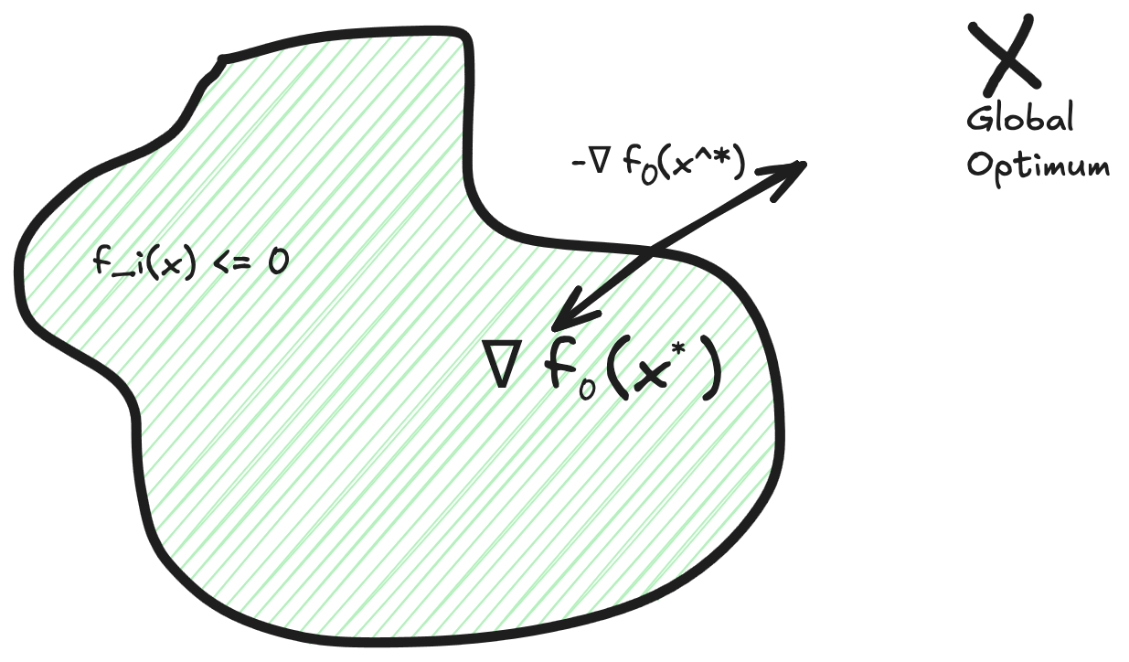
Always have the above picture in mind
The gradients are parallel to one another. Depending on the max/min, you would use the positive or the negative gradient. In case of the min, we have the negative gradient pointing outside the boundary and you have the gradient of the inequalities pointing inwards.
If the direction of lambda is flipped then this relation gets flipped.
This also has the effect of making $\lambda=0$ when $x^*$ is inside the feasible set.
KKT condition for optimality
If $x^, \lambda^, \nu^*$ are optimal then the following conditions hold
- $f_i(x^*) \le 0\qq\forall i$
- $h_j(x^*) = 0\qq\forall j$
- $\lambda^*_i \ge 0$
- $\lambda_i f_i (x^*) = 0$
- $\nabla_x f_0(x^) + \sum_i^m \lambda_i^ \nabla f_i(x^) + \sum_j^p \nu_j^ \nabla h_j(x^*)=0$
Notice the direction of the implication. If you have an optimal point then these are true. These being true doesn’t necessarily mean that the point is optimal.
But it is very useful when used in the contrapositive sense, if these conditions are not true, then the point is surely not optimal. Particularly, conditions 4 and 5 are very useful in disproving.
Specific case
If we have a convex optimization problem as our primal problem, then it is actually an $\iff$.
Perturbation analysis
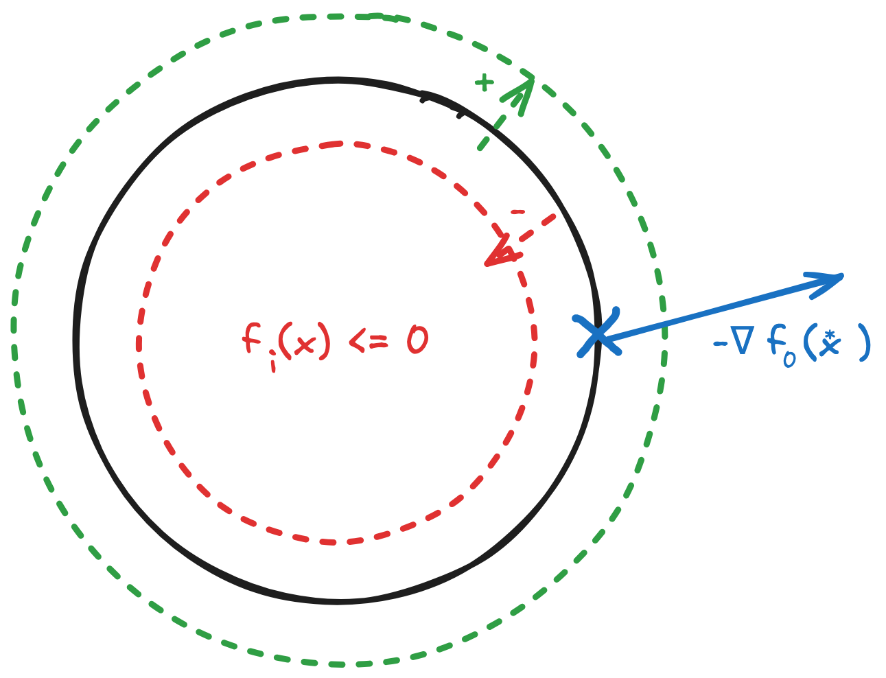
Suppose you had the above optimization problem. How to we get a sense of how sensitive the optimal value is when we change the constraints?
Let us assume that strong duality holds. We write the new optimization problem as $$ \begin{flalign} \text{minimize}\qq & f_o(x)\ \text{subject to}\qq & f_i(x) \le u_i\ & h_j(x) = v_j \end{flalign} $$
Here $u_i, v_j \in \R$. Notice that they are just affine shifts of the original constraints.
We denote the optimal value of this as $p^\star(u, v)$.
Notice that the optimal value of the original problem then becomes $p^\star = p^\star(0, 0)$
Since we have strong duality, we can say that
$$ p^\star(0, 0) = p^\star = g^\star(\lambda^\star, \nu^\star)\ = \inf_x{ f_o(x) + \sum_i \lambda^\star_i f_i(x) + \sum_j \nu^\star_i h_j(x)}\ \le f_o(x) + \sum_i \lambda^\star_i f_i(x) + \sum_j \nu^\star_i h_j(x)\ \le f_o(x) + \lambda^{\star T} u + \nu^{\star T}v\ f_0(x) \ge p^\star(0, 0) - \lambda^{\star T} u - \nu^{\star T}v\ \implies p^\star(u, v) \ge p^\star(0, 0) - \lambda^{\star T} u - \nu^{\star T}v $$
And hence the optimal points of the original dual problem serve as the sensitivity indicators of the new problem.
Particularly, they establish the lower bound on the new optimal value in terms of the unperturbed optimal value.
Interpretations
Suppose you have some unperturbed problem that you solved and found $\lambda^\star$ and $\nu^\star$. You are now going to perturb them by choosing values of $u$ and $v$. What would happen to the new optimal value?
We already know that $\lambda \succeq 0$, then
- If $u < 0$ then $-\lambda^{\star T} u \ge 0$, which would increase $p^\star$
- If $u < 0$ then $-\lambda^{\star T} u \lt 0$ which merely lowers the bound without giving any information on $p^\star$
As $\nu$ is unconstrained, we have to look at the product $\nu^T v$
- If $-\nu^Tv > 0$ which would increase $p^\star$
- If $-\nu^Tv < 0$ nothing much can be said
Local sensitivity
TODO(dbk)
Changes to the dual under problem reformulation
We have seen in an earlier class how we can form equivalent problem through certain transformations. What happens to the dual under those circumstances?
Unconstrained Problem
Suppose we have an unconstrained problem of the following form $$ \text{minimize}\qq f_0(Ax + b) $$
Its dual is the same as the primal. We cannot do anything useful with this.
Suppose we reformulate this problem as $$ \begin{flalign} \text{minimize}\qq& f_0(y)\ \text{subject to}\qq&Ax+b=y\ \end{flalign} $$
Then we formulate the dual as $$ g(\nu) = \inf_{x, y}{f_0(y) + \nu^T(Ax+b-y)}\ = \inf_{x, y}{f_0(y) + \nu^TAx-\nu^Ty} + b^T\nu\ $$
We are a pickle now. $x$ is not constrained. If $\nu^TA <0$ then the dual just keeps going down if $\nu^TA$ is anything but 0. Hence, we have to constrain $\nu^TA = 0$
Notice what this resembles. This is the conjugate of $f$
Then we have $$ \max_{\text{s.t. }A^T\nu = 0} g(\nu) = f_0^*(\nu) + b^T\nu $$
Now we have an interesting dual problem. Using the results of the last section is now possible due this change of variables.