2026/09/24 Scribe
$\newcommand{R}{\mathbb{R}}$
Let us remind ourselves the convexity condition of a differentiable function $$f(y) \ge f(x) + \nabla f(x)^T (y-x), \forall x, y$$
The best thing about convex functions is that finding where the gradient is equal to 0 gives us the global minimum. But in convex optimization problems, the situation is not so simple. We might find that the optimum point, where $\nabla f(x) = 0$, is not in the feasible set.
What do we do in that case?
The nature of convexity still helps us out. The solution must be on the boundaries.
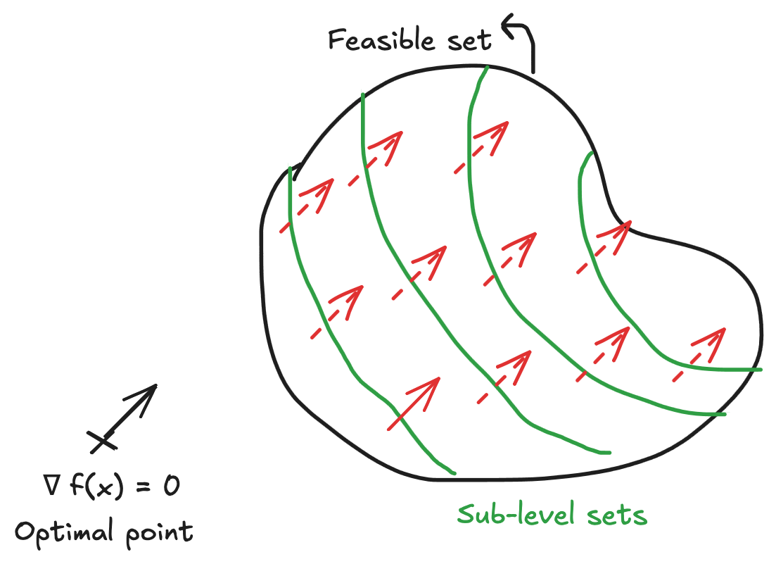
The above image illustrates the predicament we’re in. The optimal point is not feasible. But by the nature of convexity we can still deduce that the gradient must be flowing in the same direction inside the feasible set. That means that the minimum point must be at the start (Since gradient points in the direction of greatest ascent, the starting points must be smaller than all successive ones).
For some $x$ in the feasible set who is also the local minima, $\nabla f(x)$ forms a supporting hyperplane to the feasible set at $x$
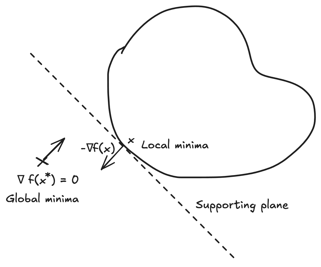
The optimum will never be inside the feasible set unless $\nabla f(x) = 0$ is inside the feasible set. The proof is pretty easy to visualize geometrically. Think of a log put into the feasible set. The log flows along $-\nabla f$. The log stop if it either reaches a minimum or the boundaries of the feasible set. If $\nabla f \ne0$ inside the feasible set, then the log will always flow and stop at the boundary.
Lagrange Multipliers have the same picture.
We can summarize this using a case analysis
- $\exists x \in C, \nabla f(x) = 0$, the optimal point is also feasible
- If $f(x)$ can be unbounded below then we won’t have any solution. This only happens when $C$ itself is unbounded which would look like $C =\mathrm{dom} f$
- $\exists x \in \partial C$ (boundary of $C$) such that $-\nabla f(x)$ defines the normal vector for a supporting hyperplane, then $x$ is the solution.
- $x$ doesn’t have to be unique
- For a polyhedron-esque feasible set, there are infinite solutions
Linear Programs
If we strengthen (weaken in terms of solving difficulty) the convexity to a linearity, we get our first class of optimization problems - Linear optimization problems.
The have the following general form $$\min c^Tx = d$$ subject to $$Gx -h \preceq 0$$ $$Ax - b = 0$$ Where $G\in\R^{m\times n}, h\in\R^m, A\in\R^{p\times n},b\in\R^p$
You may notice that these constraints are all affine rather than linear - they all have some constant shift from the origin. Then why do we call this linear programming and not affine programming? That is because the solution to the affine problems is the same as their linear counterpart. The shift don’t change the feasible set or the optimum point. Hence we can just solve the linear case to find the solution for any affine shift.
This is the simplest convex optimization problem but it is ubiquitous. It is closely linked to dual linear problem.
The word programming has no relation to computer programming. It is because it was the word that the US Military used for training and logistic schedules. Danzig, who we’ll see later, who also invented the Simplex Method to solve these, worked in the military to develop these programs, hence the name.
Usually LP $\in O(e^x)\in\mathbf{EXP}$. So it can be prohibitively expensive sometimes.
We don’t know if LP $\stackrel{?}{\in}$ strongly poly.
How to solve this?
- The feasible set of a LP is a convex polytope - higher dimensional analogue of a polyhedron.
- As we say above, the solution must lie on the boundary.
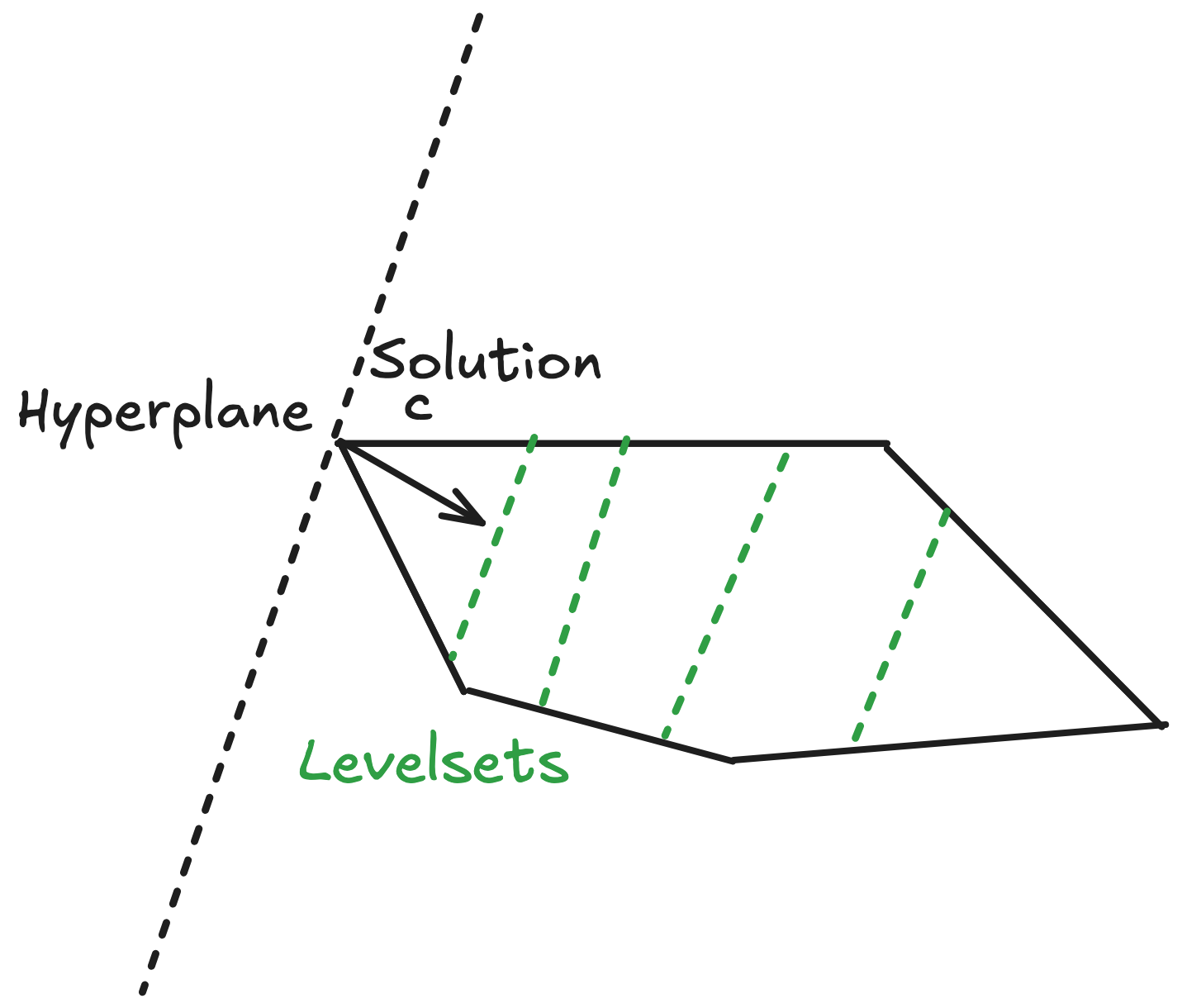
- The algorithm’s gist is that we guess vertex and move through its neighbors. Higher dimensions can cause the number of vertices to explode but linearity helps.
Standard LP
$$\min c^Tx = d$$ subject to $$Ax = b$$ $$x \preceq 0$$
We simply require the input to be in the positive orthant.