cvxopt scribe
$\newcommand{\R}{\mathbb{R}}$
Portions for the quiz
We will be covering Ch.2 Convex Sets and Ch. 3 Convex functions
Convex set
- Definition
- Affine set
- Examples of convex sets
- Operators preserving convexity
- Separating plane theorem
- Symmetric positive semi-definite, Generalized inequalities
- These are already covered under the examples but it is being pointed out to highlight their importane
- Cones
Convex function
- Definition
- 1st and 2nd derivative conditions
- Examples
- Operations that preserve convexity
- Sublevel sets
- This can be used to show non-convexity by contradiction
- Remember that this is a one way implication
- If the function is convex $\rightarrow$ all its sub-level sets are convex
- If all the convex sub-level sets $\centernot\implies$ the function is convex
- Epigraph
Convex Optimization Problem
Let us remind ourselves the form of a convex optimization problem
- $\min f : C \subseteq \R^n \rightarrow \R$ subject to
- $g_i(x) \le 0, i=1,\ldots, m$
- $h_j(x) = 0, j=1,\ldots, p$
These functions need to posses certain properties
- $f$ needs to be a convex function
- $\forall i, g_i$ is convex
- $\forall j, h_j$ is affine
- $h_j = a_j^T x + b_j$
- $a_j \in \R^n$
- $b_j \in \R$
Why do we like convex optimization problems?
- The first derivative gives you global bounds
- If $\nabla f = 0$ at some x then by the first derivative condition of $f(y) \ge f(x) + \nabla f(x)^T (y - x), \forall y$
- This is not at all possible for any old function.
Transformations
Now we are going to discuss transformations to the problem itself that preserves it convex status. We’ve seen operations that preserve convex sets, convex functions and now we’re gonna see operations that preserve convex optimization problems.
These transformations can be applied to any function. Nothing is stopping you from doing that. But we don’t really care about cases that are not convex.
Change of variables
Lets suppose we have a function that changes our input vectors into a different base,
$\phi: U \subseteq\R^n \rightarrow \R^n$ (1-to-1, aka injective and $C\subseteq \phi(U)$)
We define these new functions
- $\tilde{f} = f(\phi(x))$
- $\tilde{g_i} = g_i(\phi(x))$
- $\tilde{h_i} = h_i(\phi(x))$
Then we can reformulate our problem as
- $\min \tilde{f(z)}$
- $\tilde{g_i}(z) \le 0, i=1,\ldots,m$
- $\tilde{h_i}(z) = 0, j=1,\ldots,p$
Notice that we didn’t change anything about the solution. If $x^$ was the solution to the original problem then $z^ = \phi(x^)$ is the solution for the new problem. The opposite is also true. If $z^$ is the solution for the new problem, then $x^* = \phi^{-1}(z^*)$ is the solution for the new problem.
This is because of how we defined $\phi$. It is one-to-one and all $x$ have a valid transformation.
Transformation of objective and constraint functions
We have transformed the variables in the above section, what about transformation to the functions themselves? More precisely, can we compose the standard convex optimization problem with other functions?
Lets suppose we have the following set of functions
- $\chi: \R \rightarrow \R$
- $\phi: \R \rightarrow \R$
- $\psi: \R \rightarrow \R$
We then compose them as follows
- $\chi(f(x))$
- $\phi(g_i(x))$
- $\psi(h_j(x))$
We can use the composition rules to derive the desired characteristics of $\chi, \phi, \psi$
We know that $h\circ g$ is convex only if $g$ is convex and $h$ is monotonically increasing. Hence $\chi$ must be a monotonically increasing function.
$\phi_i(u) \le 0 \iff u\le0$
$\psi_j(u) = 0 \iff u = 0$
These just derive from substituting the values of the constraint functions.
Notice that a solution $x^$ still solves the new problem and a solution $z^$ still solves the older one.
You might have also noticed that these functions don’t really depend on $f, g, h$. Meaning none of the desired characteristics is tied to the specifics of $f, g, h$. Hence it is possible to have an entire toolbox of these $\chi, \phi, \psi$-s that can be used to transform any problem.
Example 1: Example
$f(x) = ||Ax-b||_z$
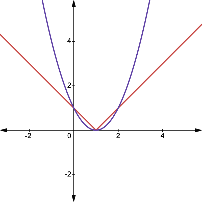
Consider the least norm solution to some linear transformation. Take the $l^1$ norm, absolute value, of this function. We know that it is not smooth.
We can smoothen it by just taking the square
$\tilde{f}(x) = ||Ax-b||_z^2$
Epigraph Problem Form
Let us remind ourselves what the epigraph of a function is
$\mathbf{epi} f =\{(x, t) | f(x) \le t \}$
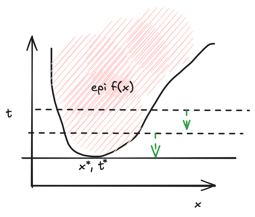
Here $t$ represents some hyperplane that cuts through the graph space. To find the minimum point, we minimize this $t$ until we barely scrape the surface of the graph.
Mathematically, the new formulation becomes
- $\min t$
- $f(x) - t \le 0$
- $g_i(x) - t \le 0$
- $h_j(x) = 0$
Notice that the new function is linear in $t$
Optimizing over some variables
So far we’ve only had one variable (though it may be in $\R^n$). What if we had two independent variables?
$\min f(x, y)$
This can be transformed into
$\displaystyle \min_{x} \tilde{f}(x)$ where $\tilde{f}(x) = \displaystyle\inf_{y} f(x, y)$
what this is saying is that an optimization problem over multiple variables can be broken down into a bunch of optimization over a single variable problems
Concretely, lets suppose we had some function $f(x_1, x_2) : \R^{n_1}\times \R^{n_2}\rightarrow \R$
There is nothing special about splitting your inputs into two variables vs having one long vector. The difference comes in the constraint functions. You can have constraint functions that are independent to one another.
- $\min f(x_1, x_2)$
- subject to
- $g_i(x_1) \le 0$
- $\tilde{g}_i(x_2) \le 0$
- $h_i(x_1) = 0$
- $\tilde{h}_i(x_2) = 0$
$\tilde{f}(x) = \inf \{f(x, z) | z\text{ satisfies all the constraints of }x_2\}$
Then the original problem is equivalent to $\min \tilde{f}(x)$ such that $x$ satisfies all the constraints of $x_1$
Abstract Convex Optimization
$f: \R^2 \rightarrow \R$
$f(x_1, x_2) = x_1^2 + x_2^2$ such that
$g(x) = \frac{x_1}{1+x_2^2} \le 0$
$h(x) = (x_1 + x_2)^2 = 0$
$h$ is not affine and $g$ is not convex. This is not a convex optimization problem. BUT, if you solve for the constraints you notice that the feasible set is still convex.
We can write new constraints as
$\tilde{g} = x_1 \le 0$
$\tilde{h} = x_1 + x_2 = 0$
These are clearly convex
Notice that the feasible set hasn’t changed. But the functions constraining it have.
What if $x^*$ is not feasible?
We know that the nice thing about convex functions is that finding a local minimum suffices to solving the problem i.e local minima is the global minima
But what happens if $x^*$ is not feasible?
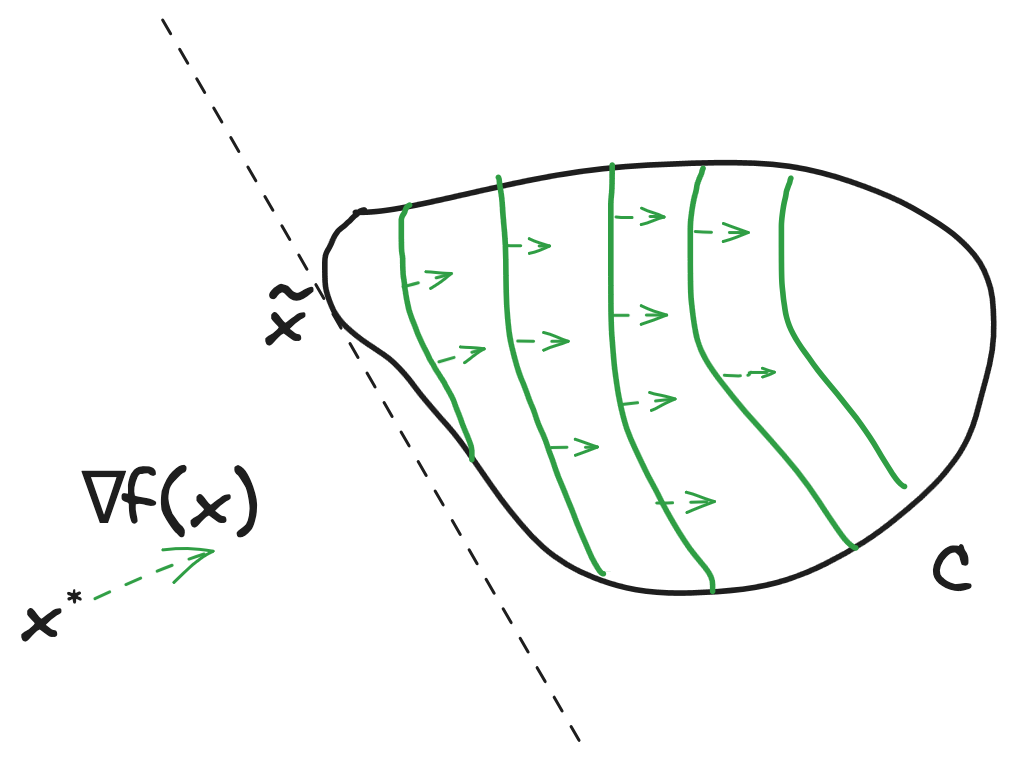
The best possible $x$ will lie on the boundary of the convex set.
This is because the gradient inside the convex set will flow in one direction. This means the minimum has to be on the boundary else the first derivative condition will be broken.
This is related to Lagrange Multipliers