2026-08-27 cvxopt scribe
$\newcommand{\R}{\mathbb{R}}$
Let us review what optimization problem really means?
We have some objective function $$ f: \R^n \rightarrow \R $$ that we want to minimize
We aren’t particularly interested in what the value of $f$ really is, as long as it it the minimum. What we really care about is $x^* = \arg \min f(x)$
We also have constraints on what values $x$ can take via the following
$$ g_i : \R^n \rightarrow \R, g_i(x) \le 0, i \in [m] $$ $$ h_j : \R^n \rightarrow \R, h_j(x) = 0, j \in [p] $$
Without some knowledge about the characteristics of $f$, this task is basically impossible. Even knowing continuity, differentiability will not help, as we say in last class.
But knowing some characteristic goes a long way. This is one of the reasons we like convexity. Just knowing that a function is convex helps out tremendously. Many IRL situations are also convex which also helps the case for being interested in convexity.
But non-convexity doesn’t automatically mean do cannot do anything. Almost all ML training objective functions are not convex yet we still optimize them.
Why always min?
- As you would have noticed that though the topic name is optimization we almost always do minimization. Why?
- In reality, it is just for the sake of convenience. Any maximization problem can be converted to minimizing its negative
- Similarly the equations for constraints can be scaled, translated without changing the canonical form.
- Greater than constraints are just negations of $g_i$
Geometric interpretation of constraints
Suppose we have some vector space $\R^n$. The equality constraint is just a hyperplane(I have drawn it squiggly to exaggerate the higher dimension. But essentially it is just a hyperplane). It just drops down the dimension by one
- The inequality constraints divide the space into two
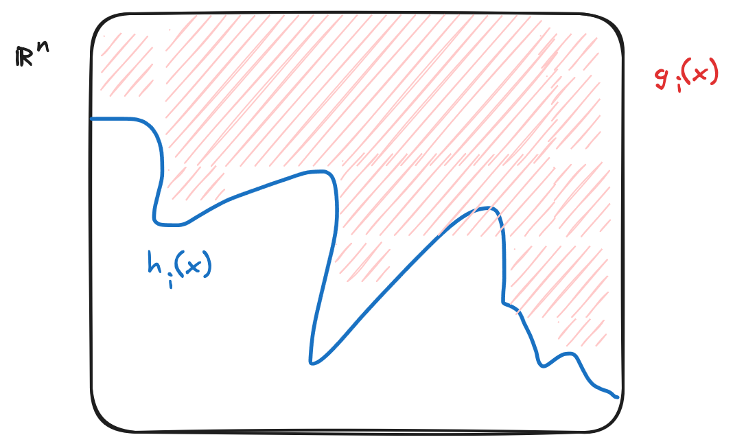
- Though geometry is optional, it is highly recommended to think of these problems geometrically. It gives you the intuition.
- The constraints are then
ANDed together. This translates to shading in a region of the graph.
What happens when nothing satisfies this?
- Then there is no solution
- A priori there is no way to know if we have a solution
Least squares
- One of the oldest studied optimization problem is least squares
- This is when the objective function is of the form $f(x) = ||Ax - b||^2_2 = \Sigma_{i=1}^m (a_i^Tx - b_i)^2$
- Here $A \in \R^{m\times n}, x \in \R^n, b\in \R^m$
- There are no constraints
Application
- The first application is Linear regression. This is attributed to Gauss.
- The way we are able to apply this is by interpreting that the errors are distributed in a gaussian fashion. This makes it that the maximum log likelihood takes the form of Least squares.
- You can also fit a polynomial instead of just a straight line
- If $A$ is full rank then we are guaranteed a closed form solution.
Linear Programming
- The second subclass of convex optimization that is very popular is $$ \min f(x) = c^Tx, c \in \R^n$$ $$= \Sigma_i^{n} c_ix_i$$
- We must have constraints for LP
- Without constraints this problem is moota
- Look at the structure of $f$. It is just like a straight line
- In $\R^n$ it will form a hyperplane that slope towards $-\infty$. So there is no way to minimize it without any constraints.
- Notice that they function itself cannot box off regions. It should be valid for all $\R^n$. It is the constraints that will box off regions and make us find solutions in some region.
- The constraints will result in a polytope
- The constraints here form an affine space instead of a hyperplane
- This is because we may not cross the zero vector and hence cannot be a hyperplane
- Unfortunately (or fortunately) linear programming doesn’t have closed form solutions. They always require iteration.
- Dantzing’s simplex method
- Interior Point method
- The solution is almost always on the boundary
- Think about it. Our $f$ is linear. It is a hyperplane. It slopes someway or the other. The solution can never in the middle. We can always find a point on the downward slope. So the solution has to be in the boundary.
- Furthermore, it mostly lies on the vertices.
Mathematical prereq.
Norm
- Norm is defined as follows $$ ||\cdot|| : \R^N \rightarrow \R $$
- Norm sort of gives us the length of a vector in some space
- It should have the following characteristics
- Non-Negativity
- $||x|| \ge 0, \forall x \in \R^n$
- Definite
- $||x|| = 0 \textbf{ iff } x = 0$
- homogeneity
- $||\alpha x|| = |\alpha| ||x||, \forall \alpha \in \R, \forall x\in\R^n$
- Linear-ish
- We need the
absbecause if the co-efficient is negative then we would break non-negativity rule
- Triangle inequality
- $||a + b|| \le ||a|| + ||b||$
- Non-Negativity
- using Norm we can define another function $d: \R^n \times \R^n \rightarrow \R$ which gives us distance
- $d(x, y) = || y - x ||$
There can be several norms for a given space. If a function satisfies the above constraints then it can be a norm. Let us see some examples of norms
L-2 norm (Euclidean norm)
$||x||_2 = \sqrt{x_1^2 + \ldots + x_n^2} = \sqrt{x^tx} = \sqrt{\langle x, x \rangle_2}$
Cauchy-Schwarz inequality
$|\langle x, y \rangle| \le ||x||||y||$
- This is because the inner product is a projection and the projections are always smaller than the original
L-1 norm
$||x||_1 = |x_1| + \ldots + |x_n|$
Any ML model that induces sparsity will require us to minimize the L-1 norm
L-p norm
As you can catch on to the pattern, we can define this for any p
$||x||_p = \sqrt[p]{|x_1^p|+\ldots+ |x_n^p|}$
L-$\infty$ norm
As we take the limit of $p \rightarrow \infty$ we get the infinite norm
$||x||_{infty} = \sup {|x_1|, |x_2|, \ldots, |x_n|}$
Unit balls of all the norms
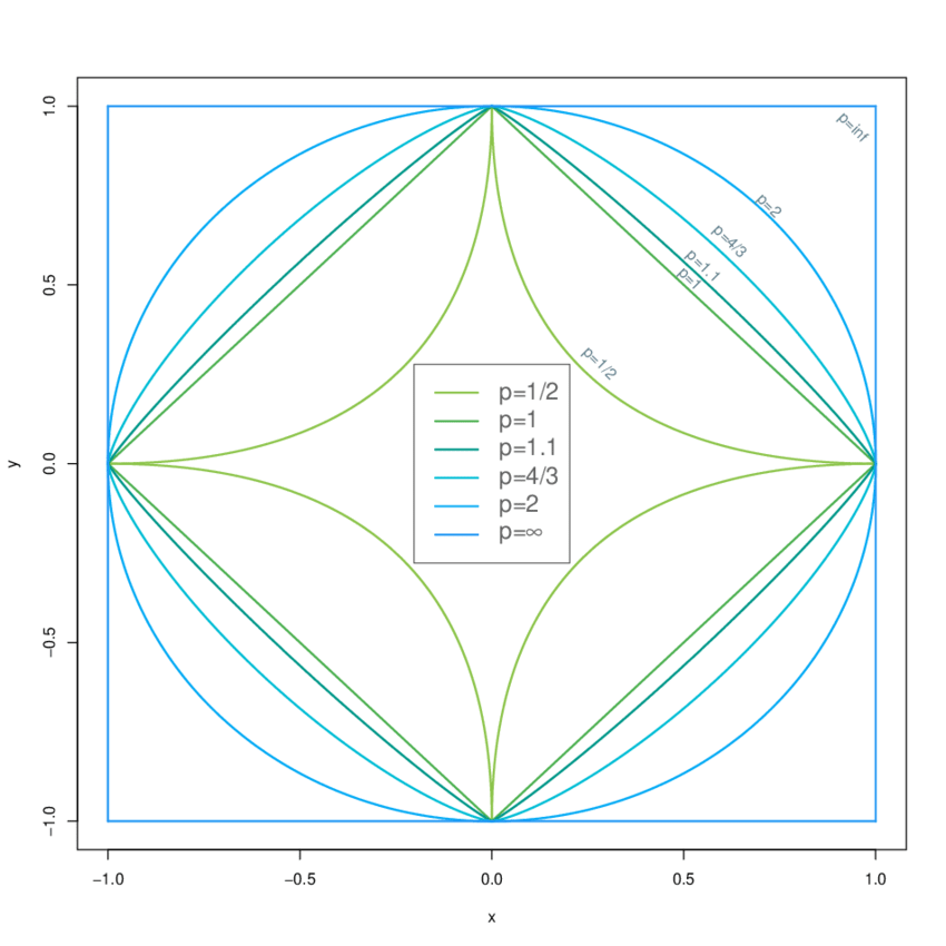 from doi:10.48550/arXiv.2003.10482
Non-integer norm
- < 1 will violate the properties