2026-02-18 Geometry of Data Scribe Notes
Shape manifolds
Goals
- Represent shapes as point on a manifold
- The shapes themselves are not a manifold, rather we will represent them on a manifold
Why can’t we do this in $\mathbb{R}^{d}$ ?
- Because rotation, translation and scaling give us a different point. We don’t want this
- Intuitively we know that a 1000m rectangle and a 1cm rectangle are the same shape
We have already seen what tangents on a manifold mean. The tangent with velocity $\vec{v}$ on a shape manifold represents an infinitesimal perturbation on the shape
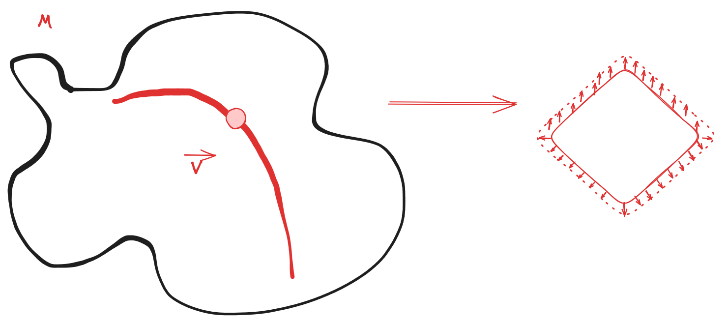
Exponential Map
- Represented as $\text{Exp}_p(\vec{v})$
- For a point $p \in M$ with a tangent vector $\vec{v} \perp p$, $\text{Exp}_p(\vec{v})$ represents the endpoint at $t=1$ on $M$
- This represents where you would end up if you start at $p$ with initial velocity $\vec{v}$ and move along the geodesic curve passing through $p$ for $||\vec{v}||$ distance
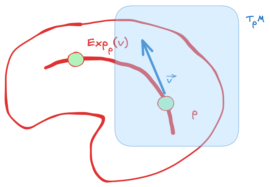
- As you can imagine we can define $\text{Exp}_p(\vec{v})$ for all possible curves passing through $p$. This is the tangent space $T_pM$.
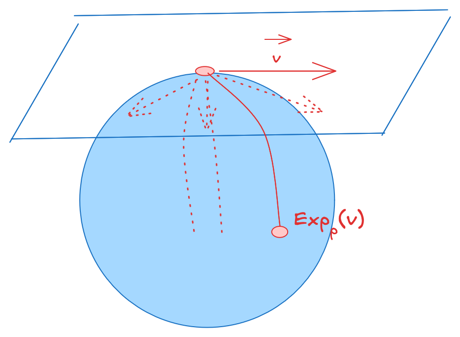
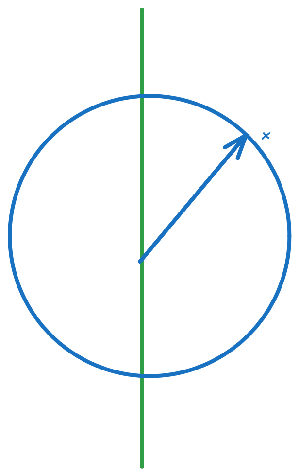
An easy example would be a sphere. Imagine the tangent space of the north pole. The set of all $\text{Exp}_p(\vec{v})$ would form a great circle just above the equator
-
In layman’s terms, tie a taunt string to the north pole of some length that is not too big and let it fall straight down. That is $\text{Exp}_p(\vec{v})$
-
The inverse of this is the Log map. This is defined everywhere except the south pole as infinite curves end at the south pole.
-
Notice the $\vec{v}$ may not be a unit vector. Normally we consider unit tangents.
-
The geodesic is a second order ODE
-
There is a theorem stating under certain conditions it is guaranteed to exist i.e for some small quantity of $t$
-
geodesic is $\partial^2$, then $\partial$ has to exist which is velocity
-
$\text{Exp}$ is guaranteed for small enough $||\vec{v}||$
- An example is $\pi$ length strings on $\mathbb{S}^2$
- $\inf$ length strings on $\mathbb{S}^2$ would result in a solution but not a unique one. You can just wrap the string around and around
-
Is there a guarantee for non-uniqueness?
- Trivial example is given above for $\mathbb{R}^d$
- Usually negative curvatures
-
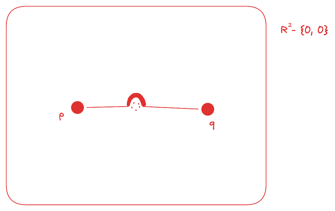
Existence is not guaranteed
-
Consider the above manifold $\mathbb{R}^2$ with ${0, 0}$ removed.
-
The distance between $p$ and $q$ are defined but there is no way to get from $p$ to $q$
-
The distance is defined as the line draw which takes infinitesimal bump over the origin
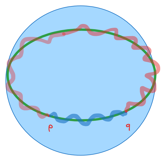
- The faint red line is the local minima between $p$ and $q$
- The faint blue line is the global minima between $p$ and $q$
Log Map
- $\text{Log}_p{q} = \vec{v}$
- This is the inverse of $\text{Exp}_p(\vec{v})$
- Returns the initial velocity
- It has to satisfy $\text{Exp}_p(\text{Log}_p(q)) = q$
- $||\text{Log}_p(q)|| = d(p, q)$
Shape Equivalence
- Let $X_1, X_2$ be some geometries
- We say that $X_1 \sim X_2$ iff $\forall \lambda, R, V, X_2 = \lambda R \cdot X_1 + V$ where $\lambda \in \mathbb{Z}_+$ , $R$ is a rotation and $V$ is translation
- This is similar to linear transformations in linear algebra
- It is clear that this $\sim$ is an equivalence relation
- It is reflexive
- It is Symmetric
- Transitive
- We denote this equivalence class as $[x] = {y : y \sim x}$
- This equivalence class partitions the space into disjoint partitions
Kendall’s Shape Space
- We define shapes to be some $k$ points in $\mathbb{R}^2$. These represent the so-called boundary of the shape. The shape has no area, volume or even continuity.
- So the entire shape will belong to $\mathbb{R}^{2k}$
- When we remove rotation, scaling and translation we will end up in $\mathbb{CP}^{k-2}$ which is a complex projective space. The name complex is sort of a misnomer as this is still homeomorphic to some $\mathbb{R}^2$
- The dimensionality reduction is due to the way we represent complex number. The point ${x, y}$ will be represented as a single $a+ib$
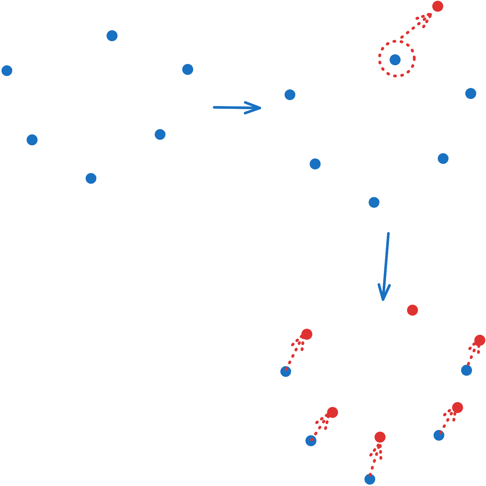
Remove scaling
- Consider the regular complex plane. The equivalence class of a point is all the rays from the origin that pass through that point.
- Mathematically we can describe this as $[x] = {\lambda \frac{\vec{x}}{||x||}: \lambda \in \mathbb{Z}-{0} }$
- $[x]\in (\mathbb{R}^2 - {0})/\mathbb{R}^+$ This is called quotient out
- We pick one point to represent each of the equivalence classes
- We get this circle centered at the origin
- We could have picked any group of points that are continuous and smooth but working with circles makes our life easy
Topological notation
- $X/\sim$ implies the set $X$ without the $\sim$ relation
- This is called quotienting out $\sim$
- Quotient space of $\mathbb{R}^d$ is $\mathbb{S}^{d-1}$
- Our object $(z_1, z_2, \ldots, z_k) \in \mathbb{C}^k$
- Removing translation will put us in $\mathbb{C}^{k-1}$
- An example is considering $z_1$ to be the origin and setting it to some constant. Then we effectively have $k-1$ $z$ coords.
- The real operation is computing the mean and subtraction from all
- $\bar{z} = \frac{1}{k}\sum_{j = 1}^{k}z_j$
- New point = ${z_j - \bar{z}: j \in [1, k]}$
- Conceptually we can think of this as the centre of mass of the point being shifted to the origin
- This is only one degree of freedom (2 in the real plane)
- $\mathbb{C}^{k-1}$ is not axis aligned
Scaling and rotation
- Since we are in the complex plane we can represent the points as $z = re^{i\phi} = (rcos\phi + risin\phi)$
- Complex multiplication of $se^{i\theta} \times re^{i\phi} = (sr)e^{i(\theta + \phi)}$
- Rotate by $\theta$ and then rotate by $\phi$
- Scale by $s$ and then scale by $r$
- This has a very simple geometric interpretation
- For our point $\mathbf{z} = (z_1, z_2, \ldots, z_{k-1})$, we have some $w \in \mathbb{C}-{0}$ and we define $[\mathbf{z}] = { (wz_1, wz_2, \ldots, wz_{k-1}) : \forall w \in \mathbb{C}-{0}}$ This represents all possible rotations and scaling
- 1-dimensional $\mathbb{C}$ is $\mathbb{R}^2$
- Ray becomes a plane in $\mathbb{R}$
- We pick one point to represent this plane
- This complex trick only works in 2-D
Actual procedure
- Represent the point using a $d\times k$ matrix. Each column corresponds to a point.
- Remove translation by $\begin{bmatrix} x - \bar{x} \\ y - \bar{y} \\ z - \bar{z}\end{bmatrix}$, subtracting mean from each row
- Remove scaling using Frobenius norm
- $||A||_F$ which essentially flattens the matrix and takes the norm
- This will put us on a sphere called the pre-shape sphere
- We remove rotation by solving the following
- $R^* = \text{arg min}_{R\in SO(d)} || RA - B ||^2$
- Where $SO$ is the special orthogonal group (rotation)
- This essentially means rotate till close to $d\times k$
- This represents a “loop” on the preshape sphere
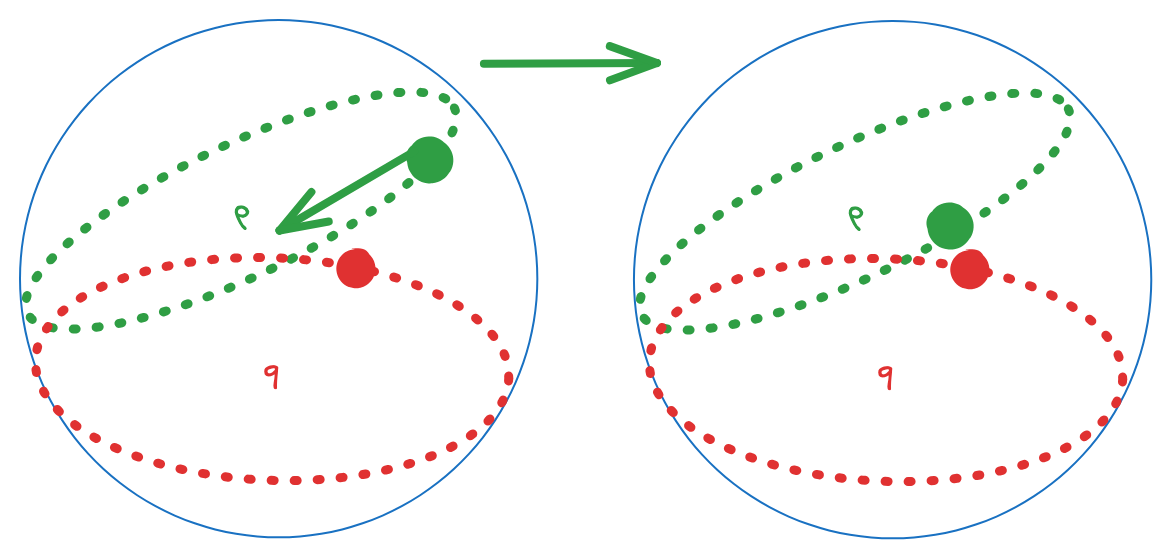 Move till alignment and then find the distance
- $U \Sigma V^T$ be SVD of $BA^T$ then $R^* = UV^T$
- Closed form solution
- Cool application of SVD
- Orthogonal Procrustes Analysis
- Why is this true?